Model Setup
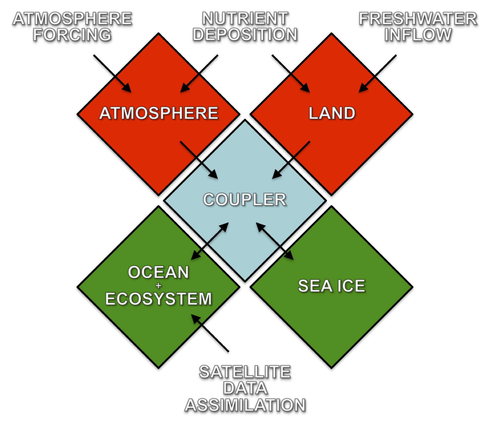
CCSM/CESM (Community Climate System Model/Community Earth System Model) is a coupled climate model that consists of five separate components with an additional central coupler (CPL7) which controls time, exchange forces, domains, grids, and other model data. The central part of this model is based on MCT (The Model Coupling Toolkit) - fully parallel coupling tools which provide many coupling services such as a component model registry, domain decomposition, descriptors, communication, data redistribution, and other beneficial tools.
For this project, CESM has been adapted for the Baltic Sea and is called 3D CEMBS. In this case, we have taken into account ocean model (POP) with ecosystem module and ice model (CICE) which are forced by atmospheric data model (DATM7).
Besides, the land model (DLND) process thg river inflow of freshwater and nutrient deposition. Other models are turned off in this configuration. The main task of the DATM7 is to interpolate forcing data on the model domain. Currently, the 48-hour atmospheric forcing data from ICM-UM model (University of Warsaw) are used.
The Ocean - POP
The ocean model is based on Los Alamos National Laboratory (LANL) Parallel Ocean Program (Smith & Gent, 2004), evolved from the global ocean model (Semptner, 1974) with added free surface formulation (Killworth et al., 1991). It is a z-level coordinate, general circulation ocean model that solves the 3-dimensional primitive equations for stratified fluid using the hydrostatic and Boussinesq approximations.
Numerically the model computes spatial derivatives in the spherical coordinates using the finite difference technique. The placement of model variables in the horizontal direction is Arakawa B-grid (Arakawa & Lamb, 1977). The barotropic equation is solved using preconditioned conjugate gradient solver (PCG), centered differencing represents advection scheme. The biharmonic operator has been chosen as a horizontal mixing parameterization and K-Profile Parametrization (KPP) to cover vertical mixing. We also use the equation of state introduced by McDougall, Wright, Jackett, and Feistel.
Sea Ice - CICE
CICE uses an elastic-viscous-plastic ice rheology (Hunke & Dukowicz, 1997). The Los Alamos CICE model is the result of an effort to develop a computationally efficient sea ice component for a fully coupled atmosphere-ice-ocean-land global climate model. It is designed to be compatible with the POP for use on massive parallel computers. CICE has several interacting components: a thermodynamic model that computes local growth rates of snow and ice due to vertical conductive, radiative and turbulent fluxes, along with snowfall; a model of ice dynamics, which predicts the velocity field of the ice pack based on a model of the material strength of the ice; a transport model that describes advection of the ice concentration, ice volume and other state variables; and a ridging parameterization that transfers ice among thickness categories based on energetic balances and rates of strain. The CICE has also multiple thickness categories and ice thickness distribution evolves over time.
Ecosystem
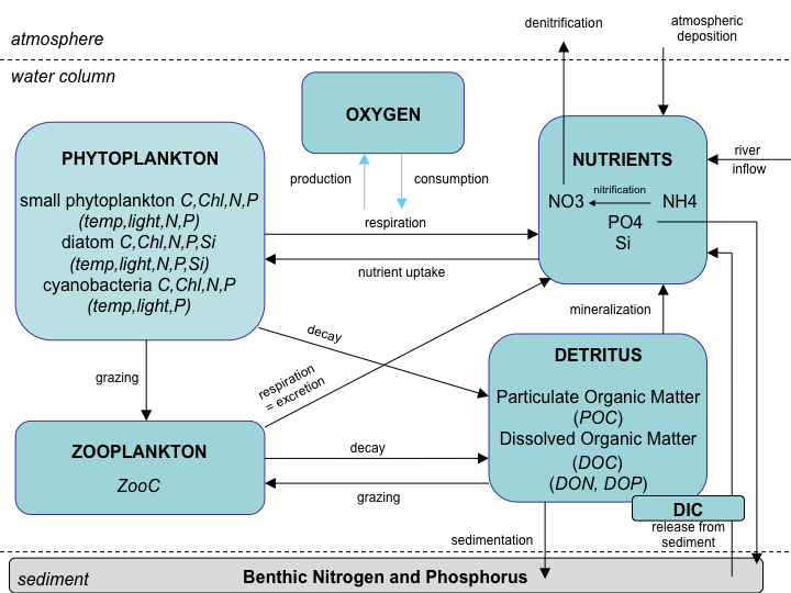
Ecosystem model (Fig. 2) is based on an intermediate complexity marine ecosystem model for the global domain (Moore et al., 2002) and consists of 11 principal components: zooplankton, small phytoplankton, large phytoplankton (mainly diatoms), summer species (mainly cyanobacteria), one detrital class, dissolved oxygen and nutrients: NO3, NH4, PO4 and SiO4.
The small phytoplankton size class is meant to represent nano- and pico-sized phytoplankton, and may is limited by nitrogen (both nitrate and ammonia), phosphate, temperature, and light. The larger phytoplankton class is explicitly modeled as diatoms and may be limited by the above factors as well as silicate. Growth rates of the cyanobacteria may be limited by phosphate, temperature, and light.
Many of the biotic and detrital compartments contain multiple elemental pools as we rack carbon, nitrogen, phosphorus, and silicon through the ecosystem. Small pelagic detritus is represented by dissolved organic carbon as well as tiny particulates.
References
- [1] Amante, C., Eakins, B.W., 2009. ETOPO1 1 Arc-Minute Global Relief Model: Procedures, Data Sources and Analysis. NOAA Technical Memorandum NESDIS NGDC-24. National Geophysical Data Center.
- [2] Arakawa, A., Lamb, V.R., 1977. Computational design of the basic dynamical process of the ucla general circulation model. Methods of Computational Physics, Vol. 17, pp. 173–265.
- [3] Hunke, E.C., Dukowicz, J.K., 1997. An Elastic-Viscous-Plastic Model for Sea Ice Dynamics. Journal of Physical Oceanography, Vol. 27, No. 9, pp. 1849–1867.
- [4] Janssen, F., Schrum, C., Backhaus, J.O., 1999. A climatological data set of temperature and salinity for the Baltic Sea and the North Sea. Deutsche Hydrographische Zeitschrift, 51(Suppl 9):5.
- [5] Moore, J.K., Doney, S.C., Kleypas, J.A., Glover, D.M., Fung, I.Y., 2002. An intermediate complexity marine ecosystem model for the global domain. Deep-Sea Res.II,49, pp. 403-462.
- [6] Seifert, T., Tauber, F., Kayser, B., 2001. A high resolution spherical grid topography of the Baltic Sea – 2nd edition. Baltic Sea Science Congress, Stockholm 25-29.
- [7] Semptner, A.J., 1974. A general circulation model for the World Ocean. UCLA Dept. of Meteorology Tech.Rep., No. 8.
- [8] Smith, R., Gent, P., 2004. Reference manual for the Parallel Ocean Program (POP). Los Alamos National Lab. New Mexico.
- [9] Stroeve, J., Holland, M.M., Meier, W., Scambos, T., Serreze, M., 2007. Arctic sea ice decline: Faster than forecast. Geophys. Res. Lett., 34.